Aug 22, 2021

The Algorithm Built to Fail

This is my entry for 3blue1brown’s first summer of math exposition (SoME1). I’m glad to report it was one of the top 100/1200+ entries and that Grant Sanderson ranked it as one of his favorite written entries!

There’s no question that elliptic curves are incredibly important to math and cryptography.


Elliptic curve cryptography spotted in Wikipedia’s security certificate

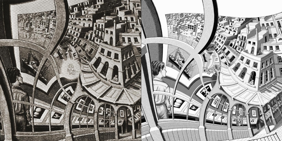
It was the key to Andrew Wiles’s famous proof of Fermat’s Last Theorem. It was even used to fill a void in one of M. C. Escher’s artworks.


Print gallery by M. C. Escher and a ‘filled-in’ version exhibiting the Droste effect

But its most creative use, in my opinion, was its application in my favorite algorithm. Strangely enough, it’s an algorithm literally built to fail. My goal is that this blog post reads like a combination of an engaging textbook and a mystery novel. By the end, I hope to give you the feeling that you could have invented this algorithm yourself by piecing together the title of this post and what you’ve learned.

By the way, the algorithm is a factoring algorithm. The goal is, given an integer, find an equivalent expression that’s a product of other integers.


A pretty good example

What are elliptic curves?

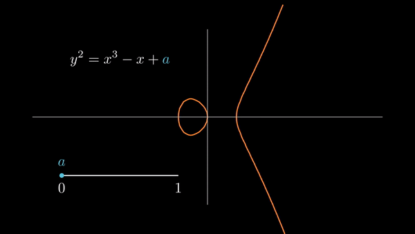
Elliptic curves consist of the solutions to

$$y^2 = x^3 + ax + b.$$


Some choices of $a$ and $b$ result in the graph having two components.

What’s interesting about elliptic curves for this algorithm is that it has

Group structure

Roughly speaking, we say that a set has a group structure if we can define an operation on all its elements which behaves like addition. That is, for a set $G$ and $+$, an operation on $G$, if

For all $a$, $b$, $c$ in $G$, we have $(a + b) + c = a + (b + c)$
There exists $0$ in $G$ such that, for every $a$ in $G$, we have $0 + a = a + 0 = a$. $0$ is known as the identity element of $G$
For each $a$ in $G$, there exists a unique $b$ in $G$ such that $a + b = b + a = 0$. $b = -a$ is known as the inverse of $a$,

then $G$ has group structure.

In the case of elliptic curves, the elements are the set of the points and the operation of choice involves first drawing a line through the points. The third point that the line passes through is denoted as the inverse of the sum. Since elliptic curves are symmetric, the inverse can be inverted by reflecting across the $x$-axis to recover the sum.


Point addition for the usual case of two distinct points

Note: If you were confused why we have to invert the third intersection previously, read the following paragraph then consider the above video animating $P + Q = R$. Rearranging this results in $P + Q - R = \mathcal{O}$. If we did not invert the third intersection, does this equation still hold?

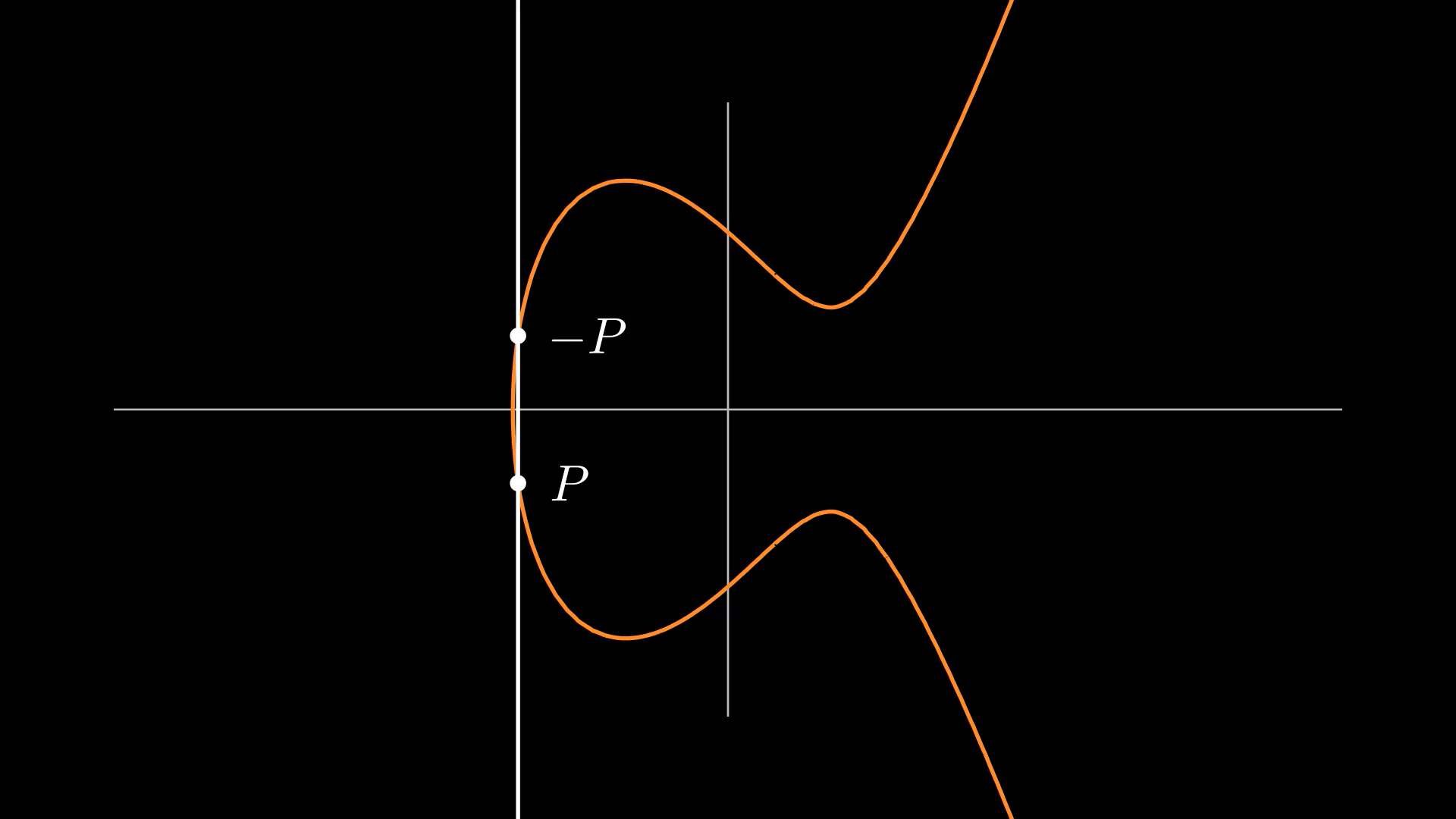
In the case of adding a point to its inverse, there’s no third intersection between the line and the curve. This leads us to define the nonexistent point ‘at infinity’ to be the identity element (denoted $\mathcal{O}$), since its sum with any other point can be defined as simply the other point, in addition to being the sum of inverses.

$$P + -P = -P + P = \mathcal{O}$$

$$P + \mathcal{O} = \mathcal{O} + P = P$$


Point at infinity not shown

Last is the case where we add a point to itself.


The drawn line is tangent to the elliptic curve

With this definition of the addition operation on the curve, we can formulate an algorithm that takes in point coordinates and returns the coordinates of the sum of the points.

Elliptic curve addition algorithm

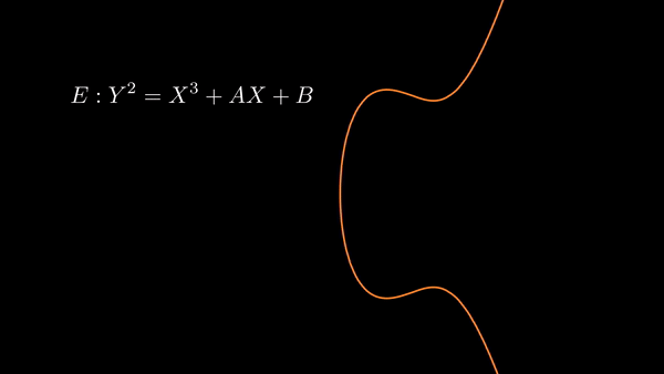
Given the curve

$$y^2 = x^3 + ax + b$$

and points $P = (x_p, y_p)$ and $Q = (x_q, y_q)$,

If $P = \mathcal{O}$, then $P + Q = Q$
If $Q = \mathcal{O}$, then $P + Q = P$
If $x_p = x_q$ and $y_p = - y_q$, then $P + Q = \mathcal{O}$. We have an undefined slope from dividing by zero, as $P$ and $Q$ have the same $x$-coordinate, resulting in a vertical line to the identity element at infinity.
Let the slope of the line through $P$ and $Q$ be

$$ \lambda = \begin{cases} \frac{y_q - y_p}{x_q - x_p} & \text{if }P \not= Q \newline \frac{3x_1^2 + a}{2y_1} & \text{if }P = Q. \end{cases} $$

The first case is the standard rise-over-run calculation of slope. The second is the slope of the tangent line computed via implicit differentiation.

Either way, we have our line

$$y = \lambda x + \nu,$$

where $\nu = y_p - \lambda x_p$ is the $y$-intercept needed to pass through $P$.

We plug this expression of $y$ into the elliptic curve equation to begin solving for the third intersection:

$$\begin{equation}(\lambda x + \nu)^2 = x^3 + ax + b.\end{equation}$$

Expanding, rearranging, and grouping terms gives

$$0 = x^3 - \lambda^2 x^2 + (a - 2\lambda \nu)x + (b - \nu^2).$$

Remember, $(1)$ was written using both the line equation and the elliptic curve equation, meaning any solution to the previous equation represents an intersection between the two. So if the third intersection is $R = (x_r, y_r)$,

$$ \begin{aligned} (x - x_p)(x - x_q)(x - x_r) &= x^3 - \lambda^2 x^2 + (a - 2\lambda \nu)x + (b - \nu^2) \newline x^3 - (x_p + x_q + x_r)x^2 + (x_q x_r + x_p x_r - x_p x_q)x + x_p x_q x_r &= x^3 - \lambda^2 x^2 + (a - 2\lambda \nu)x + (b - \nu^2). \end{aligned} $$

Notice the $x^2$ coefficients imply $x_p + x_q + x_r = \lambda^2$. We can rearrange this into $x_r = \lambda^2 - x_p - x_q$ and plug into the tangent line equation to find the corresponding $y$-coordinate.

$$ \begin{aligned} y_r &= \lambda x_r + \nu \newline &= \lambda x_r + y_p - \lambda x_p \newline &= \lambda(x_r - x_p) + y_p. \end{aligned} $$

Finally, we invert the third intersection coordinates to get our answer: $P + Q = S = (x_r, -y_r)$.

The other key detail besides the group structure of elliptic curves to consider for this algorithm is considering the curves under

Modular arithmetic


Modular arithmetic works on integers making the elliptic curve look unrecognizable

Modular arithmetic refers to the system of operating on the integers where numbers ‘wrap around’ when reaching a critical value called the modulus. In modular arithmetic, we may take expressions ‘modulo’ or ‘mod’ the modulus, meaning that we take the remainder after dividing by the modulus.

More formally, if we say that $a$ divides $b$, then there exists another integer $c$ where $ac = b$. Then in modular arithmetic, we say that $a \equiv b \mod n$ ('$a$ is congruent to $b$ mod $n$') if $n$ divides $b-a$.

For us to continue to be able to add points elliptic curves under modular arithmetic, we need to see the modular equivalents to operations in the procedure:

$$ \lambda = \begin{cases} \frac{y_q - y_p}{x_q - x_p} & \text{if }P \not= Q \newline \frac{3x_1^2 + a}{2y_1} & \text{if }P = Q. \end{cases} $$

Addition, subtraction, multiplication, and division.

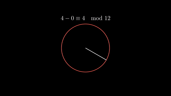
Shown below is modular addition as well as modular subtraction.


Modular arithmetic is sometimes called clock arithmetic for its familiar use in clocks

Multiplication behaves well under modular arithmetic thanks to the useful property that multiplying then $\textrm{mod}$ing is equivalent to $\textrm{mod}$ing then multiplying:

$$(a \cdot b) \mod n \equiv (a \mod n)(b \mod n) \mod n.$$

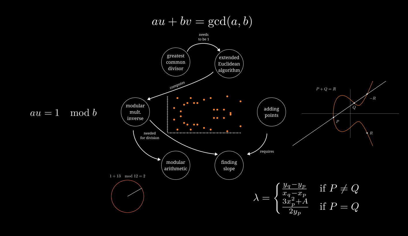
But modular division is slightly more complicated. It requires finding a number called the modular multiplicative inverse. In regular arithmetic, if we wanted to divide by 5, we could just multiply by one fifth—its reciprocal, the number to multiply to get 1. Here in modular arithmetic land, we’re going to use the extended Euclidean algorithm to find the modular multiplicative inverse and make modular division possible.

Extended Euclidean algorithm

Given integers $a$ and $b$, the extended Euclidean algorithm finds solutions to

$$\begin{equation}au + bv = \gcd(a, b),\end{equation}$$

where $\gcd(a, b)$ is the greatest common divisor (GCD) of $a$ and $b$, the largest number that divides both numbers of interest evenly. $u$ and $v$ are known as the Bézout coefficients of $a$ and $b$. When $a$ and $b$ are coprime (their $gcd$ is 1), these coefficients will give us the modular multiplicative inverse we seek.

Let’s see how it works with an example with $a = 21$ and $b = 71$. First, we compute $\gcd(a, b)$ using the regular, non-extended, Euclidean algorithm. You simply store remainder, divide, and repeat.

$$ \begin{aligned} 71 &= 3 \cdot 21 + 8 \newline 21 &= 2 \cdot 8 + 5 \newline 8 &= 1 \cdot 5 + 3 \newline 5 &= 1 \cdot 3 + 2 \newline 3 &= 1 \cdot 2 + 1 \newline 2 &= 2 \cdot 1 + 0 \newline \end{aligned} $$

Each step after

$$ \begin{aligned} b &= m_0 a + r_0 \newline a &= m_1 r_0 + r_1 \newline \end{aligned} $$

is in the general form

$$r_{i-2} = m_i r_{i-1} + r_i.$$

The remainders $r_0, r_1, r_2, \dots r_n = 8, 5, 3, \dots 0$ are non-increasing. Since we know that the last remainder is 0, $r_{n-1}$ evenly divides $r_{n-2} = m_n r_{n-1}$. $r_{n-1}$ also divides

$$ \begin{aligned} r_{n-3} &= m_{n-1} r_{n-2} + r_{n-1} \newline &= m_{n-1} (m_n r_{n-1}) + r_{n-1} \newline &= (m_{n-1} m_n + 1) r_{n-1}. \end{aligned} $$

We can continue this pattern all the way back up to show that $r_{n-1}$ divides $b$ and $a$ like a GCD should.

$$\gcd(21, 71) = 1$$

Next, we work backwards to find $u$ and $v$ from $(2)$.

$$ \begin{aligned} 8 &= 1 \cdot 71 + -3 \cdot 21 \newline 5 &= 0 \cdot 71 + 1 \cdot 21 - 2 (1 \cdot 71 + -3 \cdot 21) = -2 \cdot 71 + 7 \cdot 21 \newline 3 &= 1 \cdot 71 + -3 \cdot 21 - 1 (-2 \cdot 71 + 7 \cdot 21) = 3 \cdot 71 + -10 \cdot 21 \newline 2 &= -2 \cdot 71 + 7 \cdot 21 - 1 (3 \cdot 71 + -10 \cdot 21) = -5 \cdot 71 + 17 \cdot 21 \newline 1 &= 3 \cdot 71 + -10 \cdot 21 - 1 (-5 \cdot 71 + 17 \cdot 21) = 8 \cdot 71 + -27 \cdot 21 \end{aligned} $$

So we have $$ \begin{aligned} au + bv &= \gcd(a, b) \newline au + bv &= 1 \newline au - 1 &= -bv \newline au - 1 &\equiv 0 \mod b \newline au &\equiv 1 \mod b. \end{aligned} $$

By definition, $u$ is the modular multiplicative inverse of $a$; when multiplied with $a$ it is congruent to $1 \mod b$. In this case, -27 is the modular multiplicative inverse of 21 modulo 71.

Notice that $\gcd(a, b)$ had to be equal to 1 for this to work. Similar to regular arithmetic needing a number to be non-zero for division, modular arithmetic also has a condition for division to be defined.

Recap

At this point, you have all you need to be able to come up with a factoring algorithm using elliptic curves modulo a number. Given the context of everything you’ve learned, can you come up with an algorithm?


Goals: factor a number, fail along the way

Consider the title of this post as your final hint.

The reveal


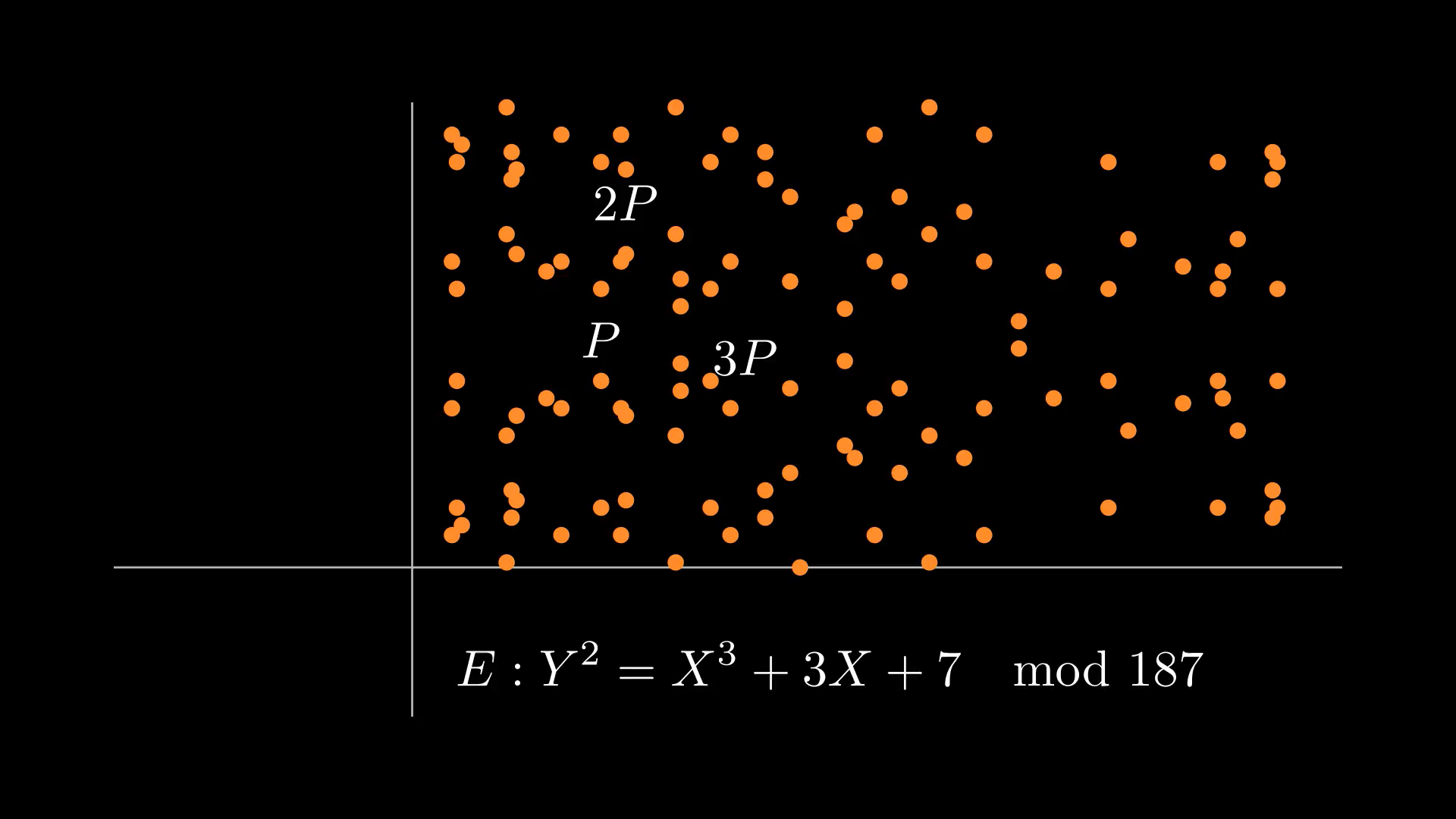
Pencil and paper ready! Can you find where division fails when we add $2P = (43, 126)$ to $3P = (54, 105)$ in the curve? Actually try it!

The key is to consider the scenario where $\gcd(a, b)$ is not 1. That would mean the extended Euclidean algorithm fails to compute a modular multiplicative inverse. We fail to divide when calculating the slope and it is undefined. If $\gcd(a, b) = c > 1$, then $c$ is a number we can use to factor $a$ or $b$, since it divides both. Our failure to divide in trying to compute a slope while adding points on the elliptic curve together results in finding a nontrivial factor! So an algorithm to factor can be trying many different curves and many different points until we encounter this scenario.

Note: In the above example, division fails when we add $2P$ to $3P$ because $5P$ is equal to the point at infinity $\mathcal{O}$ on the elliptic curve. This is because we try to divide by zero! In the world of modular arithmetic, we’ve attempted to find the multiplicative inverse of a number that’s divisible by the modulus.


Undefined slope, but due to failure to divide from dividing by zero, not $\gcd \not= 1$

Now our algorithm just needs

a way to generate elliptic curves modulo the number to be factored
a way to quickly add many points.

We can accomplish both of these by picking the coordinates of a point, defining an elliptic curve such that it contains that point, and adding that point to itself repeatedly (computing its multiples).

$$ \begin{aligned} P + P &= 2P \newline 2P + P &= 3P \newline \dots \newline (n-1)P + P &= \mathcal{O} \end{aligned} $$

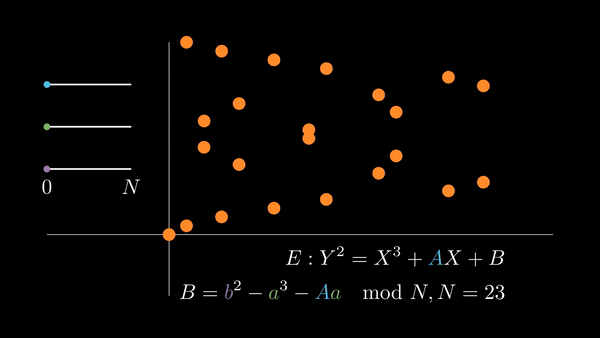
If we choose $P = (a, b)$, then pick a random $A$, we have

$$ \begin{aligned} y^2 &= x^3 + Ax + B \mod N \newline b^2 &= a^3 + Aa + B \mod N \end{aligned} $$

when we evaluate the curve at $P$. In order for $P$ to be a solution of the curve, we must have $B = b^2 - a^3 - Aa \mod N$ to satisfy the equation.


Choosing random elliptic curves

Note: in reality, it is faster to compute $n!P$ in the $n$th step of the algorithm than to repeatedly add a point to itself. This is accomplished by the double-and-add algorithm, which I will cover in the sequel post.

Conclusion

I hope you were able to reinvent this algorithm—Lenstra’s elliptic curve factorization algorithm—before its reveal.

It’s intriguing that the algorithm doesn’t just fail, but accomplishes its goal as a result of failing to compute a value. If only math tests were like that!

For part two of this series on Lenstra’s algorithm, see the next post for how Python exceptions can be used to write what might be the most intuitive implementation of the algorithm.

Anticipated questions

Why do we expect adding a point to itself repeatedly eventually become the point at infinity from dividing by zero?

You should learn about Lagrange’s theorem for more details than I will discuss here. When you have a group with finitely many elements like we do with elliptic curves modulo a number, then computing the multiples of an element by repeatedly adding it to itself will generate new points in the group, including the identity element. If you add one more multiple to the identity element, then we will be back where we started. Thus, mathematicians call the set of elements generated by doing this a cyclic subgroup of the original group. We expect this to happen because of the point’s inclusion in a cyclic subgroup:

$$H = \{ \dots \mathcal{O}, P, 2P, \dots \mathcal{O}, \dots \}$$

Who made this wonderful algorithm?

Hendrik Lenstra, a Dutch mathematician. Three of his brothers are also mathematicians, and he actually was the one who once used elliptic curves to fill the void in M. C. Escher’s Print Gallery.


“The art of doing mathematics is forgetting about the superfluous information.” —Hendrik Lenstra

How do we know that finding a factor is likely? From the last note, why is computing the factorial of a number multiples of a point instead of just adding a point to itself many times faster?

I didn’t want to drag on an already long blog post with talking about finite fields, but the answer requires knowing about them. They are algebraic objects like groups that are defined with prime numbers. Essentially, if we are trying to factor $n$ which has prime factor $p$ using point $P$, then if we look at the elliptic curve over the finite field defined by $p$, $mP = \mathcal{O}$ for some number $m$. Getting a division failure that we want from the elliptic curve $\mod n$ will happen when we compute $kP$ where $k$ is some multiple of $m$. Thus, computing a factorial multiple of $P$ will help us get there quickly. The size of the finite field depends on $p$; so if $p$ is small, then a smaller factorial multiple will get us our desired division failure. Read this for more details.

Is this algorithm the fastest factoring algorithm? Is this algorithm actually important compared to other factoring algorithms?

For general-purpose factoring, Lenstra’s algorithm is the third fastest algorithm. However, it is still in active use because how long it takes to factor does not depend on the size of the number to factor, but upon the size of its smallest factor as seen in the previous question. This makes it the fastest algorithm for large numbers which have small factors. So many factoring programs use Lenstra’s algorithm to start, then switch to more generally faster algorithms, like the quadratic or general number field sieves. Even without this utility, the algorithm is still relevant historically as it helped introduce elliptic curves to the cryptographic community, where they are now widely used.

Can I ask you a question personally?

Yes, please email me with any questions.

Where is the source code for the animations?

You can view the source code here. Apologies in advance for the messy code.

Acknowledgments

I learned this from Prof Kai-wen Lan’s MATH 5248 course at the University of Minnesota and its textbook An Introduction to Mathematical Cryptography by Hoffstein, Pipher and Silverman.

Animations are made with ManimCE and illustrations with Figma.