Happy 164th birthday, Aleksandr Lyapunov!

I recently participated in the first annual Manim math animation engine hackathon! The theme was anniversaries, so I created the above animation to celebrate the 164th anniversary of mathematician Aleksandr Lyapunov’s birth. This extended some ideas I presented from Steven Strogatz’s nonlinear dynamics textbook at the University of Minnesota’s math directed reading program symposium.

The math

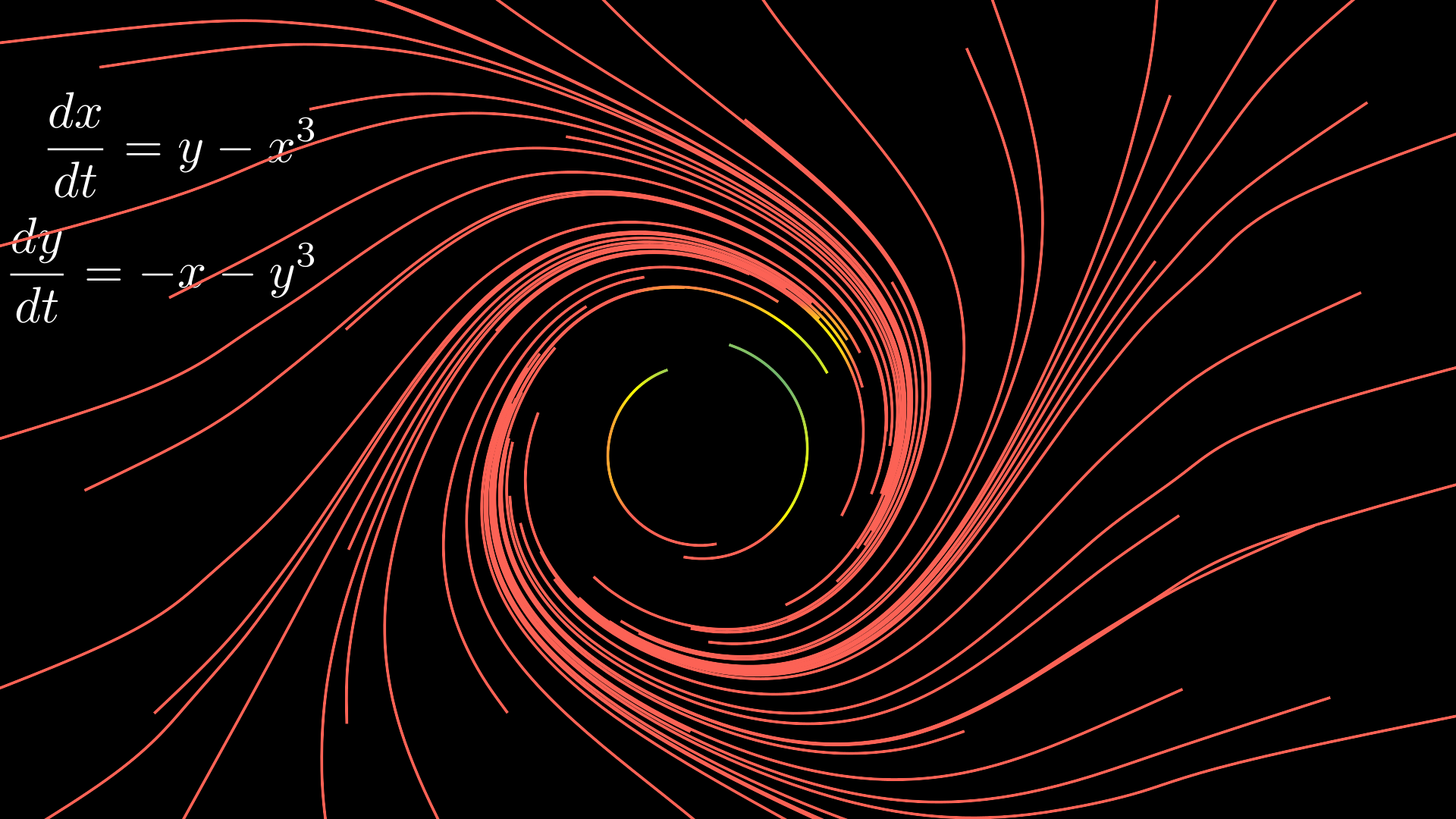
Consider the system

$$ \begin{aligned} \frac{dx}{dt} &= y-x^3 \newline \frac{dy}{dt} &= -x-y^3. \end{aligned} $$

Our dynamical system

We can’t use linearization about the fixed point at the origin to determine its stability; the Jacobian has pure imaginary eigenvalues, so the linearization is not robust to small nonlinear terms.

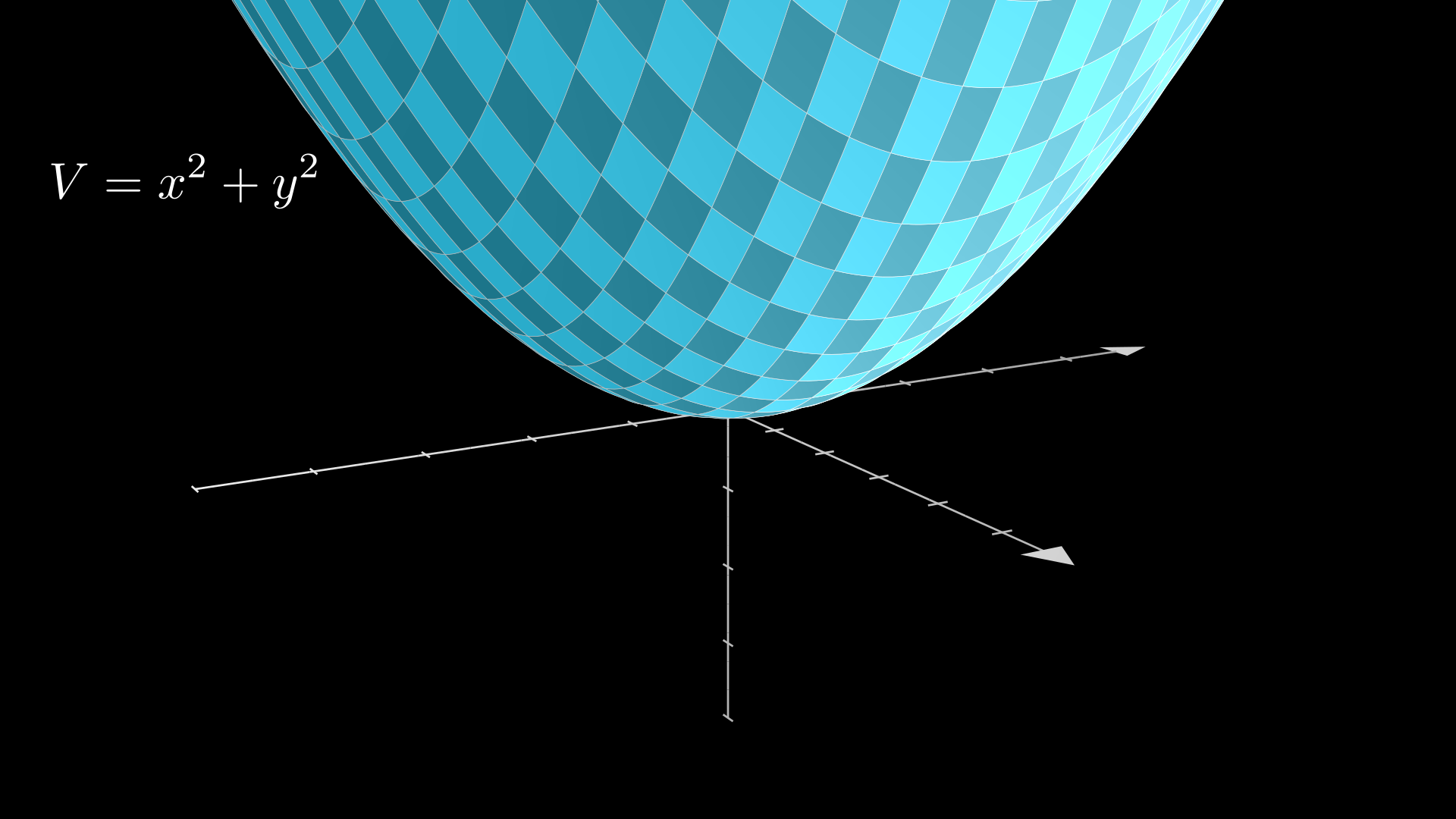
However, Lyapunov showed that finding a Lyapunov function \(V\) which is locally positive definite and has a locally negative definite time derivative implies stability. This is simimlar to an energy function as the trajectories move monotonically down the basis of \(V\). Let’s try \(V = x^2 + y^2\) for the system.

The chosen Lyapunov function

$$ \begin{aligned} \frac{dV}{dt} &= \frac{dV}{dx} \frac{dx}{dt} + \frac{dV}{dy} \frac{dy}{dt} \newline &= 2x(y-x^3) + 2y(-x-y^3) \newline &= 2xy -2x^4 - 2yx -2y^4 \newline &= -2x^4 - 2y^4 \end{aligned} $$

\(V\) is non negative and \(\frac{dV}{dt}\) is non positive, so it truly is a Lyapunov function. Its existence implies that the system is asymptotically stable; trajectories all eventually converge to the origin.

So the key insight that Lyapunov found was that there doesn’t need to be a real energy function, nor does a system have to be physical; all you need is a Lyapunov function that satisfies a few properties to determine its stability.

Outside of this toy example, Lyapunov functions are used in the engineering of nonlinear control systems. Their analogue in control-Lyapunov functions has been used in robotics for path planning around obstacles.