Jan 8, 2021

Ode to the Perceptron

If I had to explain to someone the paradigm of deep learning, I’d start by mentioning

The Perceptron

Given

$X$, an $n \times m$ matrix where each row $x$ is a data vector with $m$ features,

$w$, a vector of $m$ weights,

$b$, a bias value,

define a function $f$:

$$f(x) = \begin{cases}1 & \text{if } w \cdot x + b > 0 \\ 0 & \text{otherwise} \end{cases}$$

The task of predicting a class $d$ of some row $x$ can be solved via an iteratively improving algorithm thought to be ‘trained’ with the data in $X$. The training algorithm pseudocode is:

initialize w
define epochs
define rate
for 1...epochs
	for row x in X
		y := f(x)
		w := w + rate*(d-y)*x
	stop if w has converged


$w$ is the normal vector to the decision boundary. It is updated when there is a classification mistake i.e. when $d\not=y$. Animation code

While simple and limited (it can only achieve perfect classification when the data is linearly separable), it has many of the ingredients later used in the deep learning ‘paradigm’:

Parameters

We may think of each entry $w_i$ of $w$ as a variational parameter; $f$ behaves slightly differently for slightly different combinations of values of all the $w_i$s. In fact, $f$ can model all linear decision boundaries by varying $w$ and $b$.

There are several key differences between deep learning and perceptrons. Of course, deep learning has many more parameters, but the variation of those parameters allow them to model a much richer class of functions than just linear ones. In fact, deeps neural networks can approximately compute any function. This enables them to complete many tasks other than classification. For example, deep Q networks approximately compute the function which returns the reward given a state and an action in order to determine the optimal policy of an agent in an environment such as an Atari game.


Q-learning approximating the state-action function through the training process

Note: You might have noticed that $b$ is not changed in the training algorithm despite being a parameter. In practice, we often solve this by having $w_0$ be the bias and appending 1 as the first entry of each row $x$ in $X$.

Activation functions

Notice in the definition of $f$ that we predicted the class based on whether the sign of $w \cdot x + b$ was positive or negative. This alludes to the concept of an activation function: an operation applied on the outputs of a neuron so that its computation is not merely matrix or vector multiplication. Activation functions like sigmoid and ReLU are non-linear transformations. They are, along with using the outputs of neurons as the inputs to other neurons, what enables the aforementioned ability of deep neural networks to approximate any function.


Yup, not linear

Convergence and self-correction

The training algorithm stops when $w$ ceases to change by a certain amount with each step.

More importantly, this is achieved despite the random initialization of $w$. The training algorithm can correct mistakes during training by the vector addition

$$w := w + r(d-y)x,$$

which rotates the decision boundary in the appropriate direction, as seen in the animation. Deep learning makes a more powerful generalization to convergence and self-correction: loss functions. While linear decision boundaries can measure their performance by computing the dot product and therefore the cosine similarity of its norm and positive-class data points, we can define loss functions which establishes how well the neural network is approximating the desired function by giving a formula quantifying the mistakes in terms of $w$. Since these loss functions are differentiable with respect to our parameters, we can iteratively subtract multiples of the gradient (which gives us the change in $w$ that will maximize the loss and thus mistakes) for self-correction instead of vector addition like the perceptron does. Actually, there are a rich class of optimization algorithms based on the gradient and Hessian (a matrix of second-order derivatives) of the loss function.


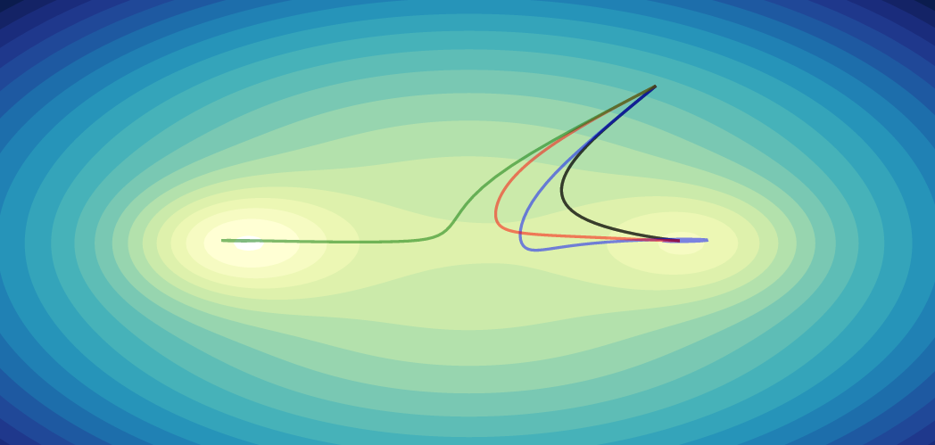Check out this wonderful visualization of optimization algorithms by Emilien Dupont

Although in retrospect it is easy to trace many of the features of the deep learning paradigm to the perceptron, this connectionist view of AI is one that was developed over several decades after Frank Rosenblatt’s original research on the perceptron. To me, it’s a fun toy example to plant the seeds in an enthusiast’s mind for the future contributions by Werbos, Rumelhart, Hopfield, McCullough, and more! The groundwork for neural networks is apparent in it; the last big idea needed was the backpropagation algorithm, which allowed for self-correction once the neurons fed their outputs as inputs to another. The concept is explained very well and at length by others, especially 3blue1brown’s video series. This intent of this post isn’t to provide a thorough explanation of the deep learning, but to highlight the historical origins of many of its ideas in the perceptron, which I don’t often see mentioned online.


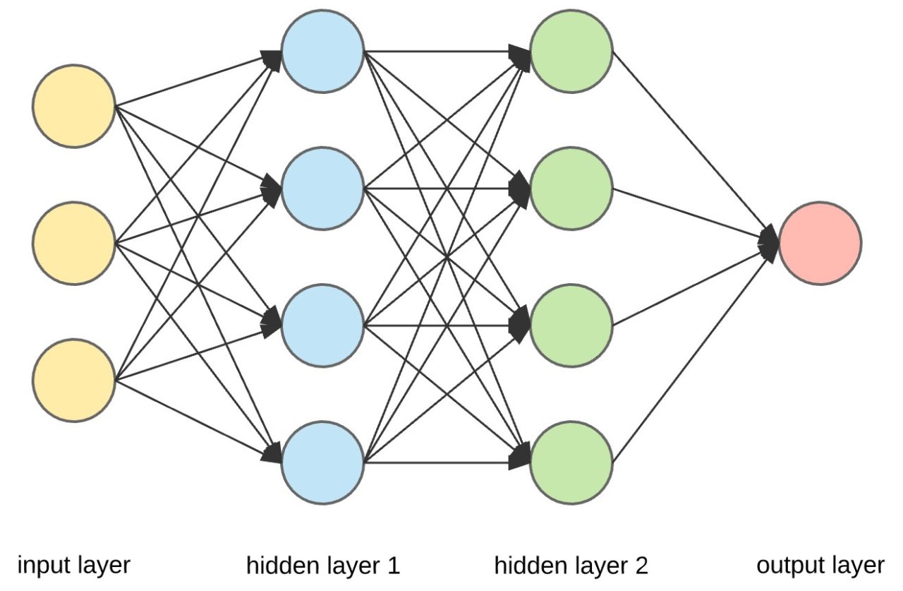A simple feed-forward neural network. Each neuron is similar to a perceptron with an activation function that uses the backpropagation algorithm to vary $w$ and correct itself. The arrows indicate the passing of outputs as inputs from one layer of neurons to the next.