Jun 17, 2020

A Segue from Segways

This content was created as part of an educational workshop for SASE Labs UMN, of which I served as director from 2020-2021. Check out the demo here.

Introduction


Polizei make Segways go brrr

Segways are pretty cool, and they can be the perfect segue into talking about control theory.

Segways need a robust mechanism for correcting itself in order to self-balance. This mechanism needs to be properly tuned and engineered so that it corrects without overshooting, delaying, or being unstable. Control theory is the study of these mechanisms.

Other examples of control systems are cruise control, process control, and thermostats.

The Inverted Pendulum

A classic system on which to test controllers is the “inverted pendulum.” It’s what you might call the “Hello World of control systems” and it’s very similar to the Segway.


An inverted pendulum

The inverted pendulum consists of a mass suspended above a pivot point. The control system must measure the angle of the pivot and move under the center of mass before the pendulum can topple down to the floor.

The Math

The output of the control system (rotating the wheels of the cart in the case of the inverted pendulum) can be described as a function.

$$u(t) = K_p e(t) + K_i \int_0^t e(\tau)d\tau + K_d \frac{de(t)}{dt}$$

where

$t$ is the current time,

$u(t)$ is the output,

$K_p$ is our tuning parameter for the proportional term,

$K_i$ is our tuning parameter for the integral term,

$K_d$ is our tuning parameter for the derivative term,

$e(t)$ is the error over time,

$\tau$ is the variable of integration which ranges from 0 to $t$.

It looks intimidating, but remember that we will have a sensor which will give us the variable to control (angle of the pendulum) in regular intervals of length $\Delta t$. This will simplify things so that our final algorithm will just be computing secant lines and Riemann sums with rectangles of width $\Delta t$.

The Algorithm

In pseudocode, the algorithm reduces to:

previous_error := 0
integral := 0

while TRUE
	error := setpoint - measured_value
	integral := integral + error*dt
	derivative := (error - previous_error)/dt
	output := Kp*error + Ki*integral + Kd*derivative
	previous_error := error
	sleep(dt)
end while

In the case of the inverted pendulum. The setpoint will be 90 degrees or $\frac{\pi}{2}$ radians because that is the pivot angle we define to have 0 error.

As you can see, the integral is computed with a left Riemann sum as the rectangles start at the first error measurement.


A left Riemann sum for varying values of $\Delta t$

When we increase our value of $K_i$, the cart holding the pendulum will move quicker proportional to the accumulated error represented by the area colored in green.

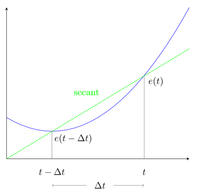
For each measurement $e(t)$ we take, we approximate the derivative by computing the slope of the secant line:

$$\frac{e(t) - e(t - \Delta t)}{\Delta t}$$


A secant line

When we increase our value of $K_d$, the cart will move quicker proportional to the rate of change of the error represented by the slope of the secant curve.

Tuning

Once we’ve programmed our cart with the PID algorithm, we still need to choose values of $K_p$, $K_i$, and $K_d$ that will balance the pendulum quickly without overshooting or being unstable.


Wikipedia has a good animation on tuning a PID

The above example shows the tuning process for maintaining a setpoint of 1. It shows how increasing $K_p$ can decrease the rise time, but lead to overshooting the setpoint. Increasing $K_i$ will shift the steady-state to the setpoint. Finally, increasing $K_d$ will provide stability.

Given our mathematical intuition relating the integral to accumulated error and the derivative to the rate of change of the error, we can come up with these general rules:

What happens when we increase …?

Parameter	Rise time	Overshoot	Settling time	Steady-state error	Stability
$K_p$	Decrease	Increase	Little change	Decrease	Decrease
$K_i$	Decrease	Increase	Increase	Eliminate	Decrease
$K_d$	Little change	Decrease	Decrease	Little change	Increase

Trying it out

Now that we know about the tuning process, let’s tune a PID on a cart-and-pole simulation.


Happy tuning!

After tuning, you can share the url in the address bar and anyone can see your personally hand-tuned PID-controlled inverted pendulum!

Next steps

Never look at Segways in the same way again
Share your very own PID!
Look at the source code
Appreciate steering wheels and thermostats a little more
Try applying reinforcement learning or genetic algorithms to the inverted pendulum problem:


Can you teach a computer to do this?

Parameter	Rise time	Overshoot	Settling time	Steady-state error	Stability
\(K_p\)	Decrease	Increase	Little change	Decrease	Decrease
\(K_i\)	Decrease	Increase	Increase	Eliminate	Decrease
\(K_d\)	Little change	Decrease	Decrease	Little change	Increase